Gun Violence Incident Grouping via PCA
Note (Oct. 14, 2016): Part of this work was used in a collaboration between the AP here and USA TODAY NETWORK here.
The Gun Violence Archive (GVA) has for each event a list of characteristics. There are 92 distinct tags that are used. Many of these tags are either redundant or unnecessarily specific for the kinds of questions I am interested in investigating:
- What are the most frequent kinds of gun-related incidents?
- Where are they located and which demographic groups are affected by them?
The mechanical issue with having so many tags is that if we treated each tag as a unique label then any statistical analysis using them is hopelessly high-dimensional. To that end a significant dimensionality reduction can be gained by using PCA to determine which groupings of tags appear frequently together; these groupings of tags will be our base level unit for categorizing gun violence events.
Encoding Tags
First we need to encode the data using one-hot encoding: every gun violence event will record either a 0 if that tag is not present or a 1 if it is. The easiest way to do this with the current system for processing data that I established in the previous post is:
- Represent each event as a python dict, with the tags as keys and the values as 1 entries. Collect all the events in a list.
- Use
scikit-learn’s excellentDictVectorizerto convert this list of dicts into a matrix where the columns correspond to a specific tag and the rows correspond to events.
After doing that, the decomposition component of scikit-learn gives us the SparsePCA function, which will be our tool of choice here. PCA determines which combinations of the original columns of the data best explain the observed variance in the data. It is these combinations which will make up our tag groupings. However, in practice normal PCA often results in every column in the original data set being used in the new description of the data. This is undesirable for our current context because we want a simple grouping of tags to jump out at us; it would do us no good if our predominant tag grouping involved in some degree all of the original tags; we would have the opposite problem where, rather than too many hyper-descriptive tags we have too few overly-general tags.
The way out of this is to use a sparse PCA algorithm, which constrains how many columns of the original data set can be used in generating principal components. From the sparse PCA algorithm we will (hopefully) achieve the goal of building robust groupings of tags based on, in some sense, their similarity to one another.
Results
The way we should interpret the results is that the algorithm has generated new, higher level tags, made up of the original tags. We have to interpret the tags now as continuous numerical quantities, not as single entries of 0 or 1. This turns out to be not so difficult of a task; we can replace the notion of a tag being present or not with simply a level of belief (my words, not a rigorous term) that this tag is appropriate for this particular event. For example, if I were to describe a particular event to you as recording in the Accidental Shooting column the value “.8”, this should be taken to mean that “more likely than not this was an accidental shooting”.
Now each bar represents a number which represents a weight on how important the individual tag is in this new tag, positive meaning “if this individual tag is present then we should have this much belief (again, not a rigorous term but just one for this explanation) in using this new tag to describe it” and negative (which is not present here but may be) meaning “if this individual tag is not present we should have this much belief in using this new tag”. The actual numerical values are not as important as the relative differences between numerical values; in other words, think of the numbers as scores attached to labels and not as actual measurements of some quantity.
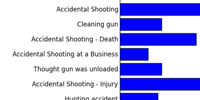
This is the first component, the one that explains the most variance in the dataset:

In plain terms, this new tag grouping is predominantly governed by the presence of the following:
- Accidental Shooting
- Accidental Shooting - Injury
- Accidental/Negligent Discharge
However, the presence of the following tags also make up nontrivial parts of this new tag:
- Accidental Shooting - Death
- Cleaning Gun
- Thought gun was unloaded
- Hunting accident
And so on, from largest weight to smallest. At this point it is up to us to give a simple label to this machine-generated hybrid tag; it seems clear to me that this is what we should take to be the “accidentally shot my gun” tag.
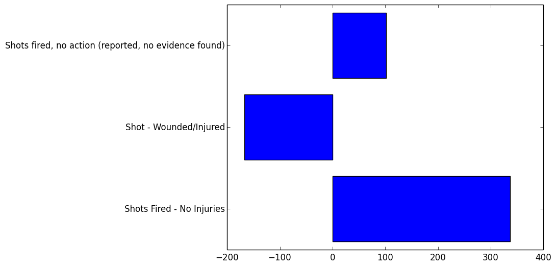
Here is the next component (the one that most explains the variance after we factor out the first component):
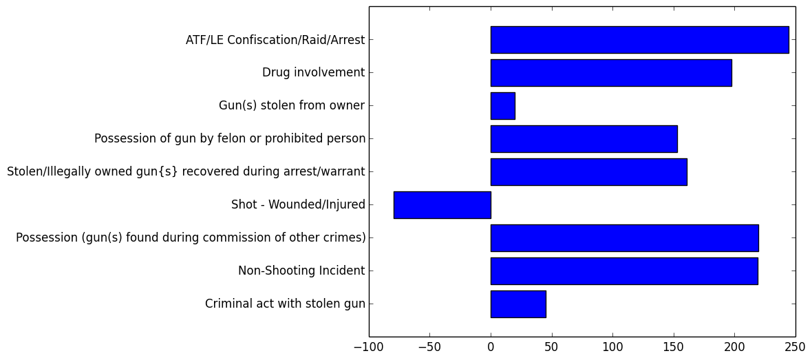
The negative weight here indicates that the lack of the Shot - Wounded/Injured is used by the component; in an interpretative sense, whenever we see Shot - Wounded/Injured we should not expect to apply our new tag and vice versa.
Looking at the remaining values, we can imagine what kind of label we should apply to this tag. In particular, the presence of the following tags lend some insight into what kind of events should carry this tag:
- ATF/LE Confiscation/Raid/Arrest
- Drug involvement
- Stolen/illegally owned gun{s} recovered during arrest/warrant
- Possession (gun(s) found during commission of other crimes)
This seems to imply we are looking at a description of “law enforcement gun recording”, what I will use to describe all of the times that guns are logged by law enforcement during the execution of their duties; specifically, the absence of any tags related to robbery, home invasion, murder seem to imply that the events that carry this tag are ones where guns are a secondary concern to the criminal activity going on (hence the strong presence of the Drug involvement tag).
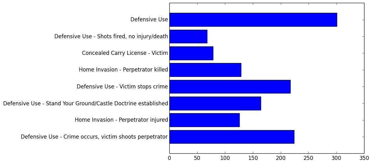
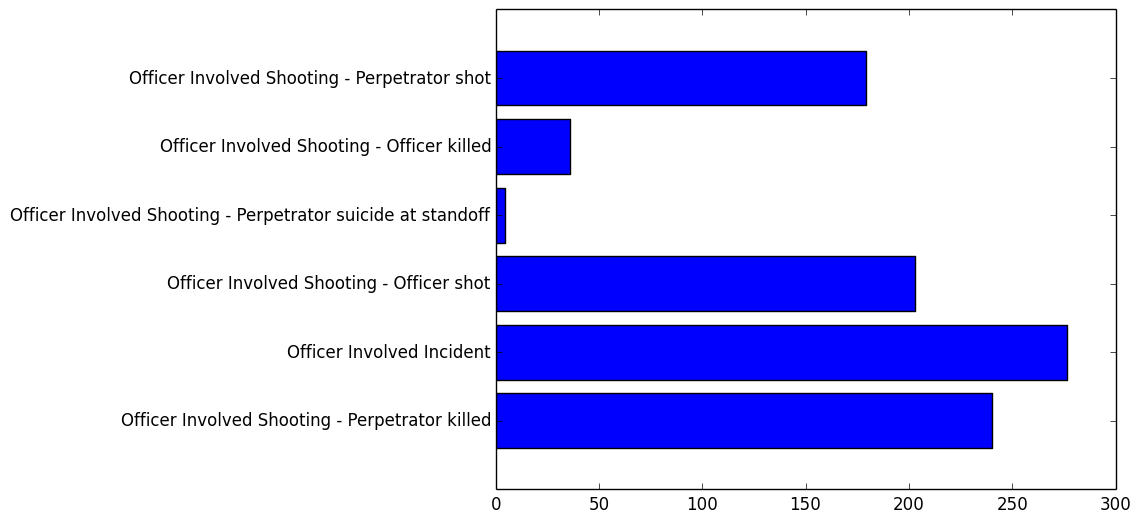
It is sometimes a fun exercise to try to interpret the principal components. Here are the remaining ones (with my idea of what they represent), down to a point where the variance explained by the component is too small to be worth talking about:
###”Successful defensive action”:
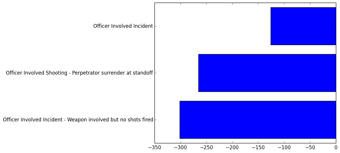
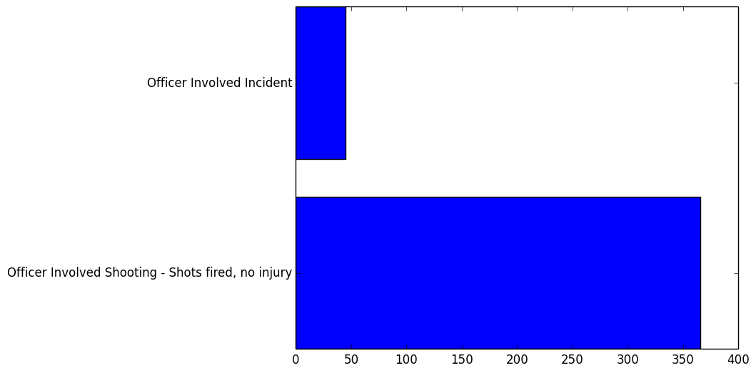
###”Police shootout”:
###”Child plays with gun”:

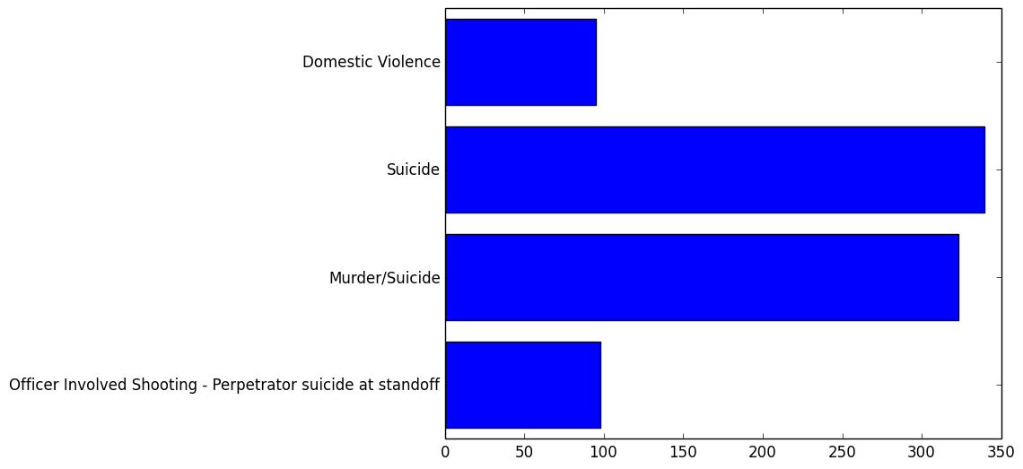
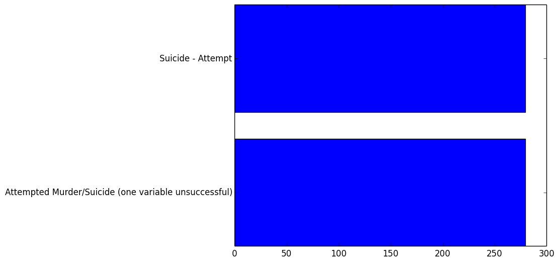
###”Premeditated murder”:
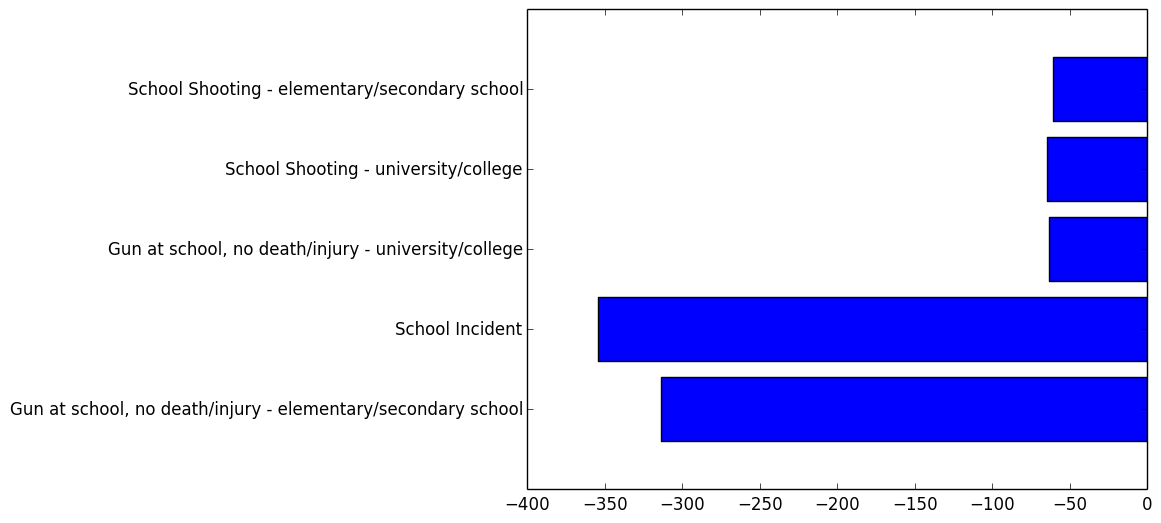
###”School safety”:
###”Home safety”:

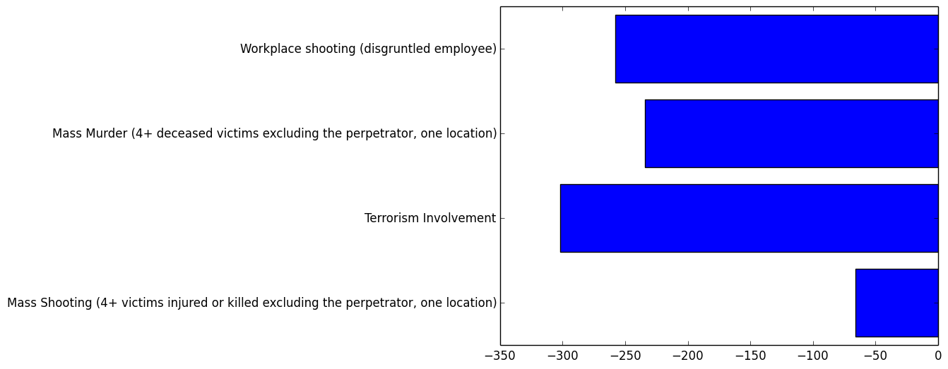
###”Public safety”:
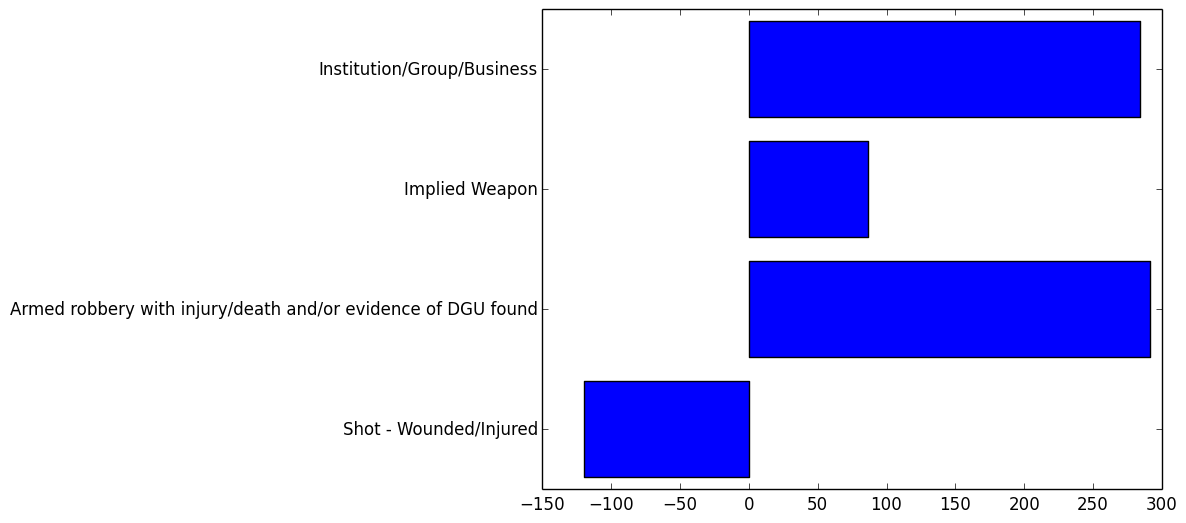
###”Bank/store robbery”:
###”Warning shots”:
Here are some of the last components we will look at. At this level there isn’t a lot of insight to be gained about how the tags group together. In some cases, it can be hard to even determine what the component represents.

Conclusion
PCA is a useful technique to reduce dimensions. Moving forward, rather than track the presence or absence of 92 separate tags I will use these generated components as references for the nine or fewer significant components I have observed. The boon is that PCA is best understood as a change in coordinates for the original data set; thus I will not lose anything by continuing my analysis using the principal components since all of the information has been preserved.